Subsetting your data
To find trends in your data, it is often necessary to subset the full data set into levels of a categorical variable. iNZight makes this easy by offering two subset by slots. Simply drag and drop variable names into them to subset the data set, or choose from the dropdown lists.
In this section, we will be subsetting (or faceting) some of the graphs we have seen previously to explore more complex relationships between variables.
Once again, we will be working with the Census at School 500 example data set we loaded in First Graphs.
Categorical Variable
We will start by creating a graph of gender by setting it as the Variable 1. If you are continuing from the previous section, you might need to clear Variable 2 by clicking the 'x' to the right of the dropdown box. You should see a bar chart of the distribution of student gender.
Now we will investigate how this distribution changes across modes of travel: drag travel to the Subset Variable 1 slot (the third box) — what do you see?
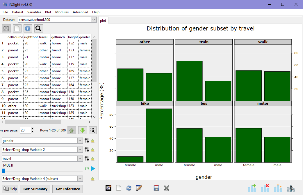
In the previous section, we looked at a two-way barplot of travel by gender: this told us about the distribution of travel by gender. This time, we are looking at the distribution of gender for each level of travel. Immediately, we can see that those students who bike to school are predominatly male, while students catching a train or bus are made up of slightly more females. Approximately equal numbers of males and females walk to school.
If you remember in the previous section we briefly mentioned a graph of gender by travel: in that case, we used travel as Variable 2 instead of Subset Variable 1. The information in these two plots is very similar, but the focus is different: in the side-by-side bar charts in the previous section, we focus on how the percent in each gender changes across modes of travel (i.e., comparing the percentage of females who bike versus who walk).
In the subsetted version, we shift our focus more explicitely to looking at how the distribution of gender changes across levels of travel. This is a tricky concept to understand, but you can easily look for yourself by switching Variable 2 with Subset Variable 1 by clicking the switch (up-down) arrows to the right of Variable 2. Compare the two graphs and think about the kind of information you can see in one that you can't in the other, and vice versa.
Numeric Variable
Sometimes you might want to see how a numeric variable influences a relationship. For example, does age affect where a student gets their lunch from? How does age affect the relationship between a student's source of model for their cellphpone and their gender? To investigate the latter, we will need to first create a graph of cellsource (Variable 1) by gender (Variable 2), and then subset by age (Subset Variable 1).
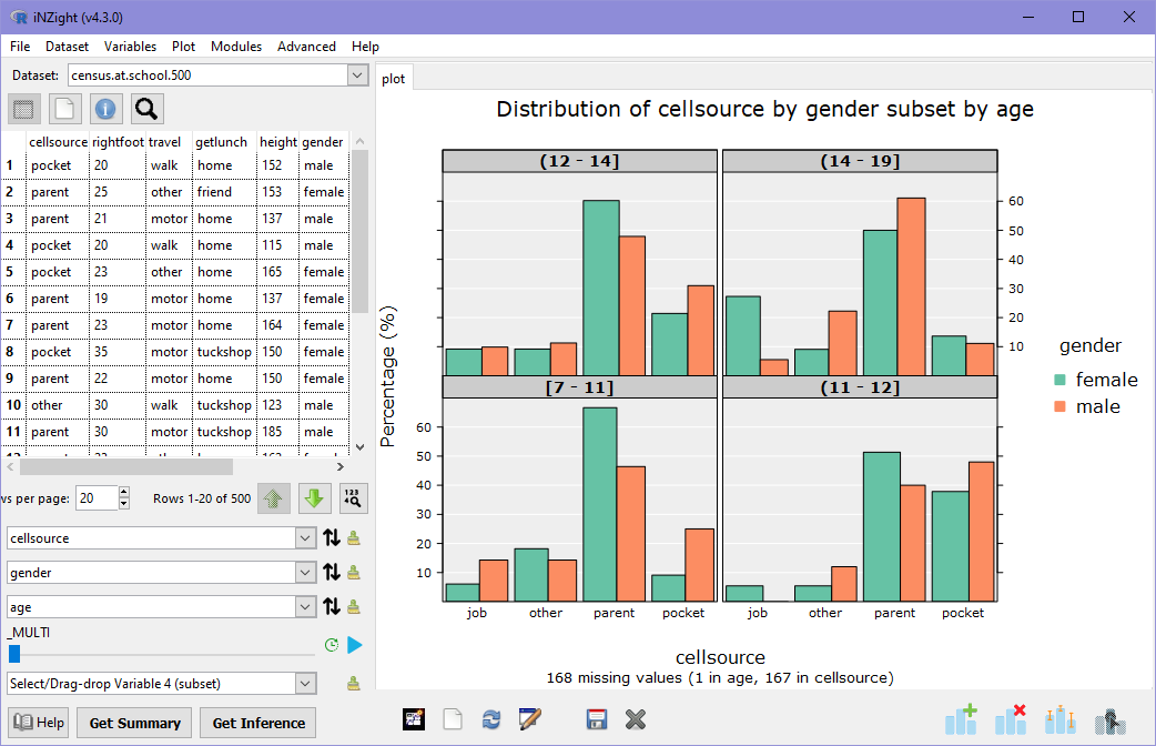
We see that iNZight has automatically split age into four groups, each with approximately the same number of observations in each. Can you spot any interesting relationships?
Look at the percentage of boys and girls using job money to pay cellphone costs: how does this change from younger to older students? If you remove gender from Variable 2, the dynamics of this relationship suddenly disappear: a few more students use job money, but we cannot see the dramatic shift for females from under 10% in the 7-11 age band up to nearly 30% in the over 14s.
To see this in action, click the Play button to the right of the slider that appeared below the Subset Variable 1 box. This will play through the subsets and show you each sequentially. Watch what happens to the distribution over time!
In the numeric subset, the age variable has been divided into groups, or intervals, and uses brackets to describe the range of each interval.
Square brackets ([]) mean that the value on that side is included in the interval, while round brackets (()) mean the value is excluded. So for example, the first interval is [7 - 11] with square brackets on both sides, so this includes students aged 7, 8, 9, 10, and 11 inclusive. The next interval, however, uses a round left bracket, (11 - 12], so this is students over 11 and up to and including 12 (which is, of course, just all students aged 12).
Where this notation becomes important is if the numeric variable can take decimal values. For example, the interval (10 - 15] can include any value greater than 10 and less than or equal to 15. It could include the value 10.2, for example, but could not contain 10. It can, however, include the value 15. An easy way to remember this is to think of the numbers as blocks — the square bracket can fit nice and snug around the number 15, but the round bracket leaves a small space between it and 10.
Subsetting by two variables
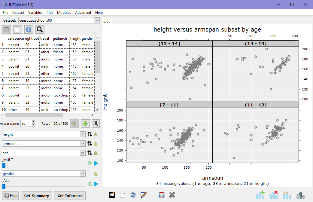
Finally, we will quickly look at how iNZight lets us explore an additional relationship by using the last box in the control panel: Subset Variable 2. This behaves a little differently that the first subsetting variable, and instead provides a look a only one level of the subset variable, rather than all at once. We will look at the relationship between height and armspan once again, this time subset by age and gender.
First, set Variable 1 to height and Variable 2 to armspan to create a scatter plot of height against armspan. Now, set Subset Variable 1 to age: you should see the plot of height against armspan by four separate age groups. Finally, set Subset Variable 2 to gender. This time, you should see no change in the graph. Here's what you should see:
In order to make use of the second subset variable, we need to use the slider. Start by dragging the slider one notch to the right ("female"). The graph should now show you the graph of height versus armspan only of females:
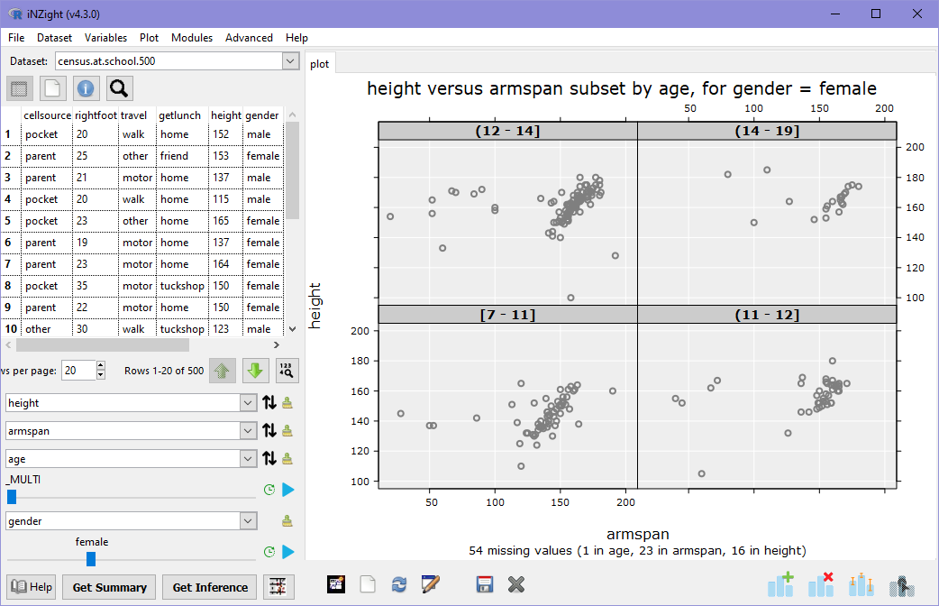
Moving the slider one place further will show only males in the plot.
Lastly, if you slide the slider all the way to the right (_MULTI), you'll see a two-way matrix, or grid, of plots for each combination of age group and gender. This can get quite messy if either (or both!) variables have lots of levels, which is why the default is to not filter at all.